So You Have Some Clusters, Now What?

How to Add Value to Your Clusters

Written by Fan Zhang, Inna Kaler

Problem

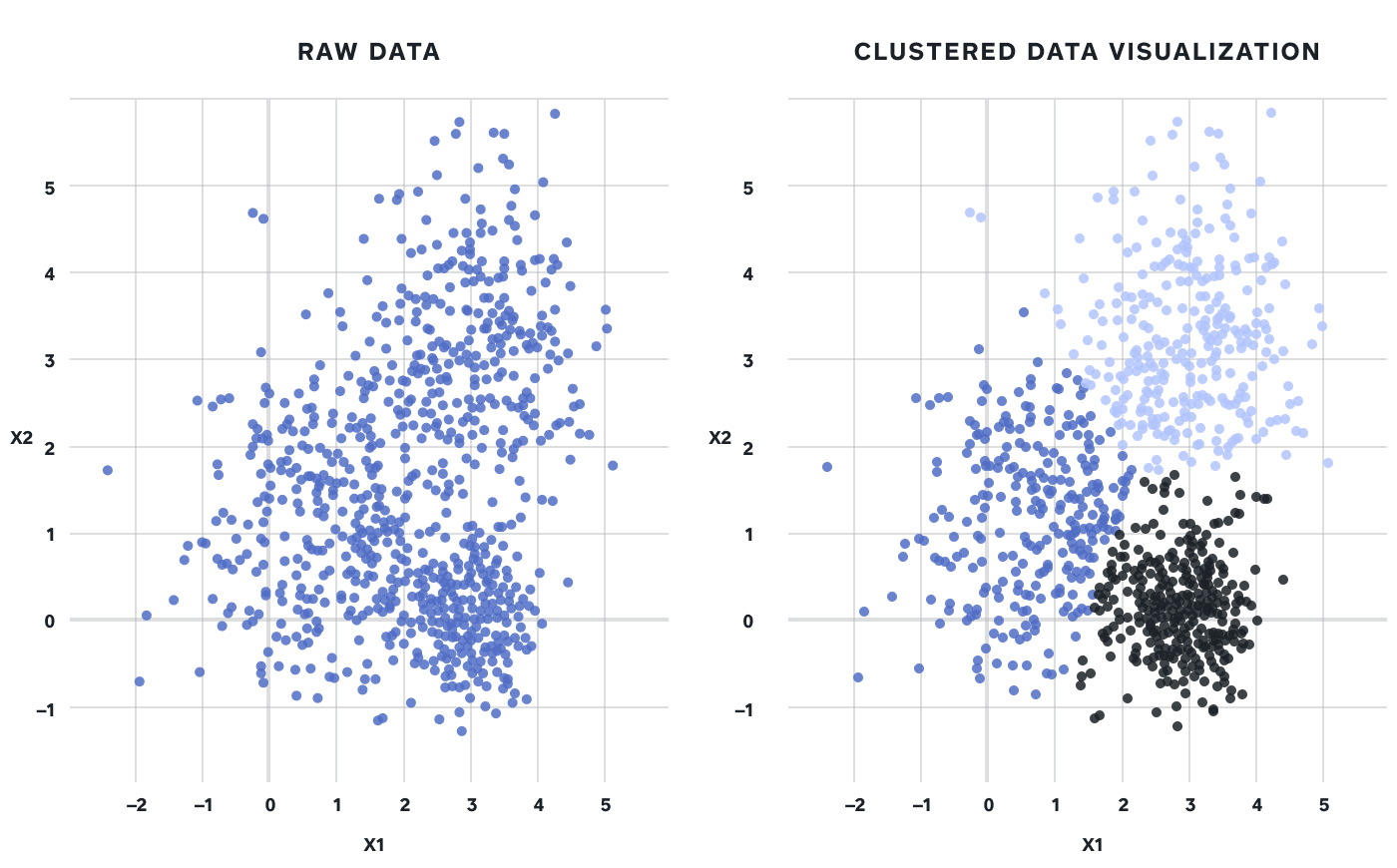
One of the most common ways to apply unsupervised learning to a dataset is clustering, specifically centroid-based clustering. Clustering takes a mass of observations and separates them into distinct groups based on similarities.

Figure 1: Taking a 2 dimensional dataset and separating it into 3 distinct clusters

For those who’ve written a clustering algorithm before, the concept of K-means and finding the optimal number of clusters using the Elbow method is likely familiar. The harder question to answer is — What does each cluster represent? We ran into precisely this problem when using clustering to understand our sellers’ behaviors.

We started out with certain assumptions about how the data would cluster without specific predictions of how many distinct groups our sellers split into. The first instinct was to manually generate a set of signals that we knew to be interesting. For example, payment volume, payment amount, and business type are some of the most common dimensions that set our sellers apart, so we attempted to use them in our clustering analysis. The resulting clusters were most optimally separated along dimensions we already knew to be important and supported our initial understanding. Retail sellers are different than Food & Drink sellers, large businesses with multiple locations are different than small single-location businesses, etc. While valuable in confirming previous understanding and analyses — this didn’t tell us anything new!

We didn’t gain any new insights about how our sellers differ because we embedded our biases of which signals are important into our dataset. So how do we get around this?

Data and Methods

To try to unlock more interesting insights, we proceeded to rebuild our clusters with a dataset containing less bias. Square’s risk systems generate thousands of signals for each seller based on a variety of behavioral signals. This is essentially the kitchen-sink of data and we used this dataset instead of hand-picking signals, which introduced the aforementioned bias. There are some reservations with this method, of course, including the possibility that we swapped known biases for unknown ones. We hope to visit this specific topic in a future blog post.

At this point, we have our data, our set of features, defined a number of K clusters, and clustered sellers into our K clusters. Next, we try a few different approaches to assign ‘profiles’ to each of our clusters:

Empirical Approach

Once we construct the clusters, we can produce a list of all sellers and which cluster they belong to. We can then take a specific cluster and study the seller characteristics along known dimensions. Alternatively, we can look at which groupings over- or under-index on specific dimensions compared to other clusters. For both approaches, we come up with a list of dimensions that differ across clusters, then make guesses on what the clusters will represent.

Here’s an example of the second approach. In this example, we joined our primary key and cluster label to the features we are interested in profiling and plotting each cluster’s average scaled value. The feature of interest is on the x-axis with the scaled average value of that feature on the y-axis. Visualizing the differences allows us to see that cluster zero is categorized by the first and last features. Meanwhile cluster three has the highest values for almost every feature profiled. From this we can start to translate nondescript cluster labels into meaningful ones explicable to an audience.

Figure 2: Average ‘score’ of each cluster along 4 different dimensions

Depending on the purpose of clustering the data, the feature set to profile clusters will change. When using clustering to understand how different sellers use a Square product, the dimensions are specific to usage data. When wanting to determine those sellers’ value to Square the feature set was comprised of broad variables related to revenue, seller size, LTV, etc.

Centroid Approach

We can figure out which seller from each cluster is the closest to the centroid (center point) and mark that seller as the most ‘representative’ seller for that cluster. We can then study the sellers along known dimensions or signals to come up with our best guess of the cluster profile as with the empirical approach. An alternative approach is to study the hypothetical centroid instead of the most representative element. For both approaches, we are making assumptions about how representation works within our groups, so which is the better approach of the two is strictly situational. Of course, if the variance within clusters are large, then neither the hypothetical nor empirical centroid would feel very representative of the group.

Here’s an example of this approach. In the graph below, the star in the middle of each cluster indicates the most representative member of the cluster.

Figure 3: Stars identify the centroid of each cluster

Supervised Learning from Cluster Membership

Once the clusters are created, we can isolate the most influential features that vary the most across the different clusters, and make an educated guess about the cluster’s profile. This is a more sophisticated version of determining how clusters are over or under-indexing.

One way to tease apart the influential features this is with a Random Forest Classifier. For example, if we have 4 clusters, we can use our existing signals to predict the probability of everyone belonging to the first cluster, then the second, etc. The result would be K models to match K clusters, one model per cluster, and predicting whether an instance is likely to belong to each cluster. Most standard implementations of the Random Forest algorithm will show you which features are important for each particular prediction, which can inspire more intuitions on what these important features says about the cluster itself.

Another way to arrive at feature influence is to use a single multiclass classification model (sklearn.multiclass) with your response as the column ‘Cluster’ with values of 1,…,K. This provides the benefit of a singular model that can be used to predict an instance’s cluster using additional signals outside the K-means dataset. For example, in the application of product usage, you could profile users into clusters without them having used the product yet to segment your addressable market more specifically. We hope to expand on this technique in a future blog post.

Results

Once we determine which dimensions mattered in separating our clusters, we are likely to find one of two things: either the top signals are not aligned with what we previously believed to be important, or that they are.

If our result is the former, then great! You can gain insights about what new behaviors your observations diverge on and how they’re different than your existing assumptions. Ideally, these divergences are significant and actionable.

More often than not, however, the top signals that the clusters split on are already known and expected. This at the very least validates that existing segmentations are meaningful, but we can learn more.

Given that your data is most optimally separated by your top signal, what if you cluster again within these clusters? This would then reveal a second set of signals that are important, controlling for the first set. We did exactly that when we discovered that our first clusters were separated into our existing segmentation of business size. We added an additional list of signals that weren’t present in our first dataset and a list of insights that clued us into how our sellers differ at various business sizes emerged. This set of insights informed strategy across marketing and product teams, and provided a personalized approach to product development and seller interactions.

When it comes to clustering, you are rarely done after you pick the optimal number of clusters and run the algorithm. There is a lot of value in the interpretability of your clusters and the additional understanding you gain of your data.